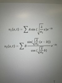
Deriving the temperature equations for a composite wall using the heat equation

[shreddinglicks]

I began by setting alpha_sub_1 and alpha_sub_2 equal to zero in my Matlab script. The results behaved as I expected which was promising.

However, when I proceeded to change the sinusoidal arguments in the spatial solutions;

making lambda become lambda/sqrt(alpha_sub_u)

where u is 1 or 2 depending on which spatial solution was being evaluated, I get crazy curves.

 

[logistic_guy]

I began by setting alpha_sub_1 and alpha_sub_2 equal to zero in my Matlab script. The results behaved as I expected which was promising.

However, when I proceeded to change the sinusoidal arguments in the spatial solutions;

making lambda become lambda/sqrt(alpha_sub_u)

where u is 1 or 2 depending on which spatial solution was being evaluated, I get crazy curves.

You should not set \(\displaystyle \alpha_1\) and \(\displaystyle \alpha_2\) to zero. If you set them to zero, it is like removing the term \(\displaystyle \frac{\partial^2 u}{\partial x^2}\) from the original differential equation.

Do you think that the problem was solved?

 

[shreddinglicks]

You should not set \(\displaystyle \alpha_1\) and \(\displaystyle \alpha_2\) to zero. If you set them to zero, it is like removing the term \(\displaystyle \frac{\partial^2 u}{\partial x^2}\) from the original differential equation.

Do you think that the problem was solved?

My apologies, I meant to say I set the alphas equal to 1. When I do that the curves produced make sense.

When the alpha values are any other number I get crazy curves that make no sense.

 

[logistic_guy]

My apologies, I meant to say I set the alphas equal to 1. When I do that the curves produced make sense.

When the alpha values are any other number I get crazy curves that make no sense.

If every condition is satisfied and the results the solutions produce make sense, it doesn't matter how crazy the curves look like.

 

[shreddinglicks]

If every condition is satisfied and the results the solutions produce make sense, it doesn't matter how crazy the curves look like.

They do not make sense. They look like squiggly noodles, not smooth curves.

 

[shreddinglicks]

I also checked the difference between having alpha in the time or spatial equation. It seems equivalent.

Also, I tried making both alphas the same value. It doesn't fix the problem.

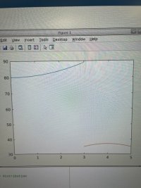
Below is the graph of the initial curves using parabolas. Both alpha values are equal to .05
k1=30
k2=18
left temperature at 80
right temperature at 35
interface is at x=3
right side x=5
Rc =.008

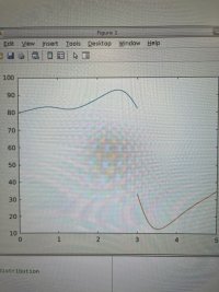
Next is the graph at t=1

The result does not make sense.

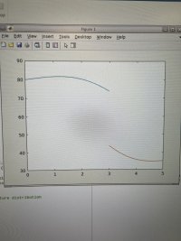
Now if I make both alphas equal 1. I get what intuition tells me.

This happens regardless of whether I put alpha in the spatial of time equation.

 

[logistic_guy]

It is very difficult to catch what was wrong (if there was any) because you chose to solve a very complicated system. I want to know the origin of this question. Did you create this problem by yourself or it was given to you by a website, a book, a teacher, or someone else?

Let us try this one last time. Choose some values for these parameters. Try to not choose the same value twice!

\(\displaystyle a\)
\(\displaystyle b\)
\(\displaystyle \alpha_1\)
\(\displaystyle \alpha_2\)
\(\displaystyle f(x)\)
\(\displaystyle P(x)\)

And any other parameters that will come later such as \(\displaystyle k_1\) and \(\displaystyle k_2\).

If you use this information, what do you get for the first three eigenvalues?

\(\displaystyle \lambda_1\)
\(\displaystyle \lambda_2\)
\(\displaystyle \lambda_3\)

 

[shreddinglicks]

I created this myself. I have been self studying on my free time. You can see my other posts on this website where I worked on other applications of the heat equation.

I will respond back with my results soon.

 

[logistic_guy]

I created this myself.

It is good to be creative, but don't blame others if the error was not found. It is like that you are the manufacturer and I am just a simple employee in your factory. If the maker cannot spot his error, don't expect the workers to see it!

Or may be your creation was not perfect and you just have not realized it yet.

 

[shreddinglicks]

It is good to be creative, but don't blame others if the error was not found. It is like that you are the manufacturer and I am just a simple employee in your factory. If the maker cannot spot his error, don't expect the workers to see it!

Or may be your creation was not perfect and you just have not realized it yet.

I'm not blaming you. I appreciate the help. It is often by talking and working with others that I accomplish my goals.

I'm going to redo the problem to ensure it is free of errors and then write back with the Matlab results.

 

[logistic_guy]

I'm not blaming you.

That's the spirit of a real sports man.

By the way I checked your spatial solutions and I thought to tell you that it would be easier for calculations to choose:

\(\displaystyle X(x) =\begin{cases}X_1(x) & 0 < x < a\\X_2(x) & a < x < b\end{cases} =\begin{cases}A\sin \lambda x & 0 < x < a\\B\sin \lambda(b - x) & a < x < b\end{cases}\)

Though there was nothing wrong with what you chose!

 

[shreddinglicks]

I did find that my script was giving me bad eigenvalues. I fixed it and it appears better but still a problem.

My values are

alpha₁ = .05
alpha₂= .03
k₁= 30
k₂= 18
a=3
b=5
R_c=.08
u₁(x,0) = x² +80
u₂(x,0) = -x² +35
The temperature at the left boundary is 80
The temperature at the right boundary is 35

lambda₁=.0383
lambda₂=.1884
lambda₃=.4833

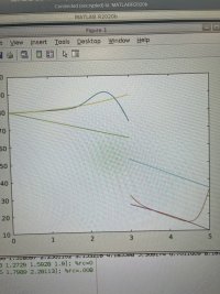
Below is the graph at t=1. The straight lines are the steady state curves. The curved lines are the transient curves. The lines the transient curves overlay partially are the initial conditions.

The transient curve to the right seems to behave well.

The transient curve on the left seems to have a strange bump around 2<x<2.7

 

[logistic_guy]

Beautiful work you did so far

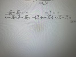
What was your equation that produced these lambdas, \(\displaystyle \lambda_1, \lambda_2, \lambda_3\)?

Why do you think that a bump in the transient solution is a strange thing?

 

[shreddinglicks]

I expect the transient curve to be lower than the initial curve for all values of t>0. The left material should be cooling when in contact with the right material which is warming.

 

[logistic_guy]

lambda₁=.0383
lambda₂=.1884
lambda₃=.4833

I checked your equation. If I use it, I get:

\(\displaystyle \lambda_1 = 0.359\)
\(\displaystyle \lambda_2 = 0.433\)
\(\displaystyle \lambda_3 = 0.686\)

I have seen you doing pretty well in finding the steady state and the transient solutions, so I will trust in you and your other calculations!

I expect the transient curve to be lower than the initial curve for all values of t>0. The left material should be cooling when in contact with the right material which is warming.

Are you an expert in curves or what? If you are, then you should already know the following:

One of these can cause a bump in the graph.

Material property mismatch:
If thermal conductivities \(\displaystyle k_1 \neq k_2\), the rate at which heat spreads in each region differs. A bump can form temporarily in the region with slower diffusion (often the less conductive material).

Contact resistance:
If there's resistance to heat flow at the interface (modelled as a discontinuity in flux or temperature), heat might "pile up" on one side (often the higher-resistance side), creating a transient local maximum.

Initial conditions:
The initial temperature distribution or mismatch in temperatures between regions can set up a scenario where a temporary bump forms and then smooths out as time progresses.

Mathematical solution behavior:
Solutions to parabolic PDEs like the heat equation can have non-monotonic transient states, especially near boundaries or interfaces with discontinuous conditions.

There are also many other factors that can cause that rise in the curve. I am as an expert in ODEs and PDEs for more than \(\displaystyle 5\) years, I expect a temporary rise (bump) develops but gradually levels out over time.

Therefore, it is very normal to see a bump, even though it may seem counterintuitive at first.

 

[shreddinglicks]

I checked your equation. If I use it, I get:

\(\displaystyle \lambda_1 = 0.359\)
\(\displaystyle \lambda_2 = 0.433\)
\(\displaystyle \lambda_3 = 0.686[/
\)

What did you use to get these eigenvalues?

 

[logistic_guy]

What did you use to get these eigenvalues?

Desmos.

 

[shreddinglicks]

I tried Desmos. I notice it connects the dots at the asymptotes and gives false zeros.

 

[logistic_guy]

I tried Desmos. I notice it connects the dots at the asymptotes and gives false zeros.

I will check it again and I will let you know!